The old company name and logo may still be indicated on products, printed materials or web site published before its change.
Those shall be read as the new ones.
| TECHNICAL INFORMATION |
| Effective Use of the Math Function Module (1) |
| Math function modules (computation units) are widely used
in various process instrumentation systems. M-System offers various kinds of modules.
The following article is to explain M-System’s procedure of gain and bias
calculation methods. Models available are M2ADS (adder), M2SBS (subtractor), JF and JFK. |
| Adder-subtractor |
 Addition-subtraction
is necessary in cases where a total value indication for liquid flow through multiple
pipelines or that of liquid level for several reservoir tanks is required. An
adder-subtractor (M-System’s Math Function Module, Model JF or JFK) is used
for this purpose. Addition-subtraction
is necessary in cases where a total value indication for liquid flow through multiple
pipelines or that of liquid level for several reservoir tanks is required. An
adder-subtractor (M-System’s Math Function Module, Model JF or JFK) is used
for this purpose.Practical application examples are shown in Figures 1, 2 and 3. Figure 1 shows an example that indicates the total liquid flow, Flow 1 + Flow 2. Figure 2 shows an example that indicates the total amount of liquid of two cylindrical reservoir tanks, Level 1 + Level 2. Figure 3 shows another example that indicates the total quantity of liquid of two spherical reservoir tanks by the help of the linearizer that is able to convert liquid level of a spherical tank to the corresponding liquid amount. The Model JFX1 is a highly accurate Linearizer that provides a 100 segment poly-gonal line approximation representing this level. |
| Gain Calculations — Addition-subtraction | |||||||
 The
Math Function Module does not have an indicator, therefore an engineering unit
scale is n ot used. Its input and output signals are limited to 4 – 20 mA
DC or 1 – 5 V DC. Computations within the module are carried out using numerical
values of 0 – 1 or 0 – 100%. When input and/or output conditions change,
the preset constants in the module must also be changed which can involve somewhat
complicated procedures. That is to say, gains and biases for the computation equation
s hould be re-calculated. In these calculations, the specific engineering unit
scalings should be used for bo th input and output signal ranges. The
Math Function Module does not have an indicator, therefore an engineering unit
scale is n ot used. Its input and output signals are limited to 4 – 20 mA
DC or 1 – 5 V DC. Computations within the module are carried out using numerical
values of 0 – 1 or 0 – 100%. When input and/or output conditions change,
the preset constants in the module must also be changed which can involve somewhat
complicated procedures. That is to say, gains and biases for the computation equation
s hould be re-calculated. In these calculations, the specific engineering unit
scalings should be used for bo th input and output signal ranges. As
a typical example, Figure 4 shows the calculation procedure for the application
shown in Figure 1. The input and output signal ranges for this example are as
follows: As
a typical example, Figure 4 shows the calculation procedure for the application
shown in Figure 1. The input and output signal ranges for this example are as
follows:
In this case, all engineering unit scales start at zero which means that bias need not be considered. Therefore, the following equation is used for the Math Function Module:
 In
most basic applications, the equation: Output = Flow 1 + Flow 2 is used. However,
in this example the output range becomes 0 – 2 using this formula, instead
of the 0 – 1 intended range. Because of this, values for gains K1 and K2 must be determined. The following equations
are used to determine their values: In
most basic applications, the equation: Output = Flow 1 + Flow 2 is used. However,
in this example the output range becomes 0 – 2 using this formula, instead
of the 0 – 1 intended range. Because of this, values for gains K1 and K2 must be determined. The following equations
are used to determine their values: The actual calculation for the example shown in Figure 4 is: 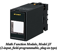 |
| Gain Calculations — Biased Signal Range | ||||||||
 An
example of gain calculations for biased signal ranges is shown in Figure 5. The
input and output signal ranges in engineering units are as follows: An
example of gain calculations for biased signal ranges is shown in Figure 5. The
input and output signal ranges in engineering units are as follows:
When both Flow 1 and Flow 2 are 0%, the following is true:
In this case, only the gains K1 and K2 need to be considered in this application. Each gain is calculated by using the following: In this example, these are calculated as follows:
|
| Output Bias Calculation | ||||
 When
the input signal range has a bias, and at the same time the output signal range
starts form zero without a bias, the math equation becomes slightly more complex.
A typical example is shown in Figure 6. The input and output signal ranges in
engineering units are as follows: When
the input signal range has a bias, and at the same time the output signal range
starts form zero without a bias, the math equation becomes slightly more complex.
A typical example is shown in Figure 6. The input and output signal ranges in
engineering units are as follows:
In this example, the output bias B in the following equation should be calculated. First, the two inputs must be added in their respective engineering units at their 0% values. The resulting bias value (B) is calculated as follows: The gains K1 and K2 are calculated in the same manner as shown in the preceding example:
|
| Input Bias Calculation | ||||||||||||
 The
example used for the output bias calculation can be also used as an example for
an input bias calculation. This is shown in Figure 7. The input and output signal
ranges in engineering units are as follows: The
example used for the output bias calculation can be also used as an example for
an input bias calculation. This is shown in Figure 7. The input and output signal
ranges in engineering units are as follows:
The following equation is used for this example:
The input bias values are calculated as follows: Then, The gains K1 and K2 are calculated easily in two steps. For Flow 1, the span (including the bias) is 200 m3/H (Range: 0 – 200 m3/H) versus the span of the actual signal, 100 m3/H (Range: 100 – 200 m3/H). The first step is to determine the value for the gain k1: Next, the output gain k2 is calculated: The resultant gain K1 can be obtained by multiplying k1 and k2 as follows: The gain K2 for Flow 2 is determined by the same procedure:
|
||||||||||||